
Agentic AI DevOps: Building Neural Network Architecture : Pytorch
Recap of the previous session
- A neuron is a small model (
m·x + bplus an activation function). A neural network arranges neurons in an input layer, hidden layers and an output layer. - Activation functions: sigmoid (binary output), softmax (multi-class output) and ReLU (hidden layers). A regression output needs none.
- Training: forward pass, loss, backward pass, update weights, repeated for many epochs.
- With a neural network, you configure the layers, neurons, loss function, learning rate and optimizer.
In this session
- When to use statistical models and when to use a neural network
- The dataset: house price prediction
- Preparing data for PyTorch: NumPy, scaling, tensors
- Building a simple network, then a network with hidden layers
- The training loop and the evaluation
- Saving the model and serving it as an API
In one sentence: you do the same steps as in statistical ML, but you build the model yourself with PyTorch and write the training loop that you theorised about.
1. Statistical model or neural network?
- If the data is small and simple, use a statistical model. It is easier.
- If the data is bigger or more complex, or unstructured, use a neural network. It also works for structured data.
The session uses simple structured data (house prices), so you can focus on the network instead of data cleaning. The dataset is already numeric, with no missing values.
2. The use case
Predict a house price from eight features: sqft, bedrooms, bathrooms, age, floors, garage, lot_size and city_index. The target is price. It is a regression problem with 1,000 records.
import pandas as pd

data = pd.read_csv("../house_data.csv")
X = data.drop(columns=["price"])     # 8 features
Y = data[["price"]]                  # the target
3. The framework: PyTorch
With statistical ML you picked a ready-made model from scikit-learn. To build a neural network you use a deep learning framework. The two popular ones are PyTorch and TensorFlow. PyTorch is the one used most in practice, and it is the one used here.
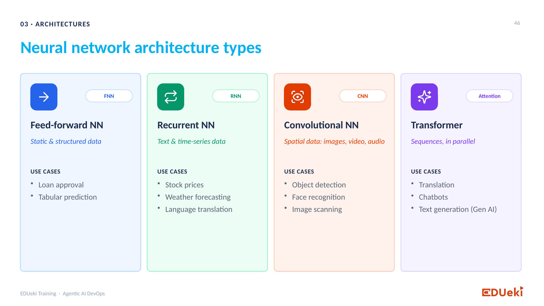
Neural network architecture types
There are different types of network, for different data:
| Type | Typical data and use |
|---|---|
| Feed-forward | Static, structured data, such as loan approval or house prices |
| Recurrent | Data that changes with time: stock prices, weather |
| Convolutional | Images, video, audio |
| Transformer | Natural language: chatbots, text generation, translation |
The transformer is the architecture behind modern LLMs and is the next big topic. The recurrent and convolutional types are not needed for this course. We use the feed-forward type here.
4. Preparing the data for PyTorch
PyTorch expects the data as tensors, a data type like a DataFrame or a NumPy array. The conversion goes in steps, after all your cleaning and feature engineering:
- DataFrame to NumPy (
float32). - Split into training and testing data.
- Scale the data with
StandardScaler. - NumPy to tensors with
torch.from_numpy.
import numpy as np
from sklearn.model_selection import train_test_split
from sklearn.preprocessing import StandardScaler
import torch

X_new = X.to_numpy(dtype=np.float32)
Y_new = Y.to_numpy(dtype=np.float32)

x_train, x_test, y_train, y_test = train_test_split(X_new, Y_new, test_size=0.2, random_state=42)

x_scalar = StandardScaler().fit(x_train)        # learns the mean and spread of each feature
y_scalar = StandardScaler().fit(y_train)

x_train_scalar = x_scalar.transform(x_train).astype(np.float32)    # now apply it
x_test_scalar  = x_scalar.transform(x_test).astype(np.float32)
y_train_scalar = y_scalar.transform(y_train).astype(np.float32)
y_test_scalar  = y_scalar.transform(y_test).astype(np.float32)

x_train_tensor = torch.from_numpy(x_train_scalar)
x_test_tensor  = torch.from_numpy(x_test_scalar)
y_train_tensor = torch.from_numpy(y_train_scalar)
y_test_tensor  = torch.from_numpy(y_test_scalar)
StandardScalerrescales each column so that the values sit on a similar, small scale (around 0). Networks train much better this way, because a column such assqftin the thousands would otherwise swamp the others..fitonly learns the scaling rule (the mean and so on)..transformapplies it to the data. That is why there are two steps.- The result is for the machine, not for you to read.
- 800 rows are for training and 200 rows for testing (an 80/20 split), each with 8 columns.
5. Building the network
Install and import PyTorch (pip install torch), then define the network as a class. nn.Sequential stacks layers one after another.
Option 1: a simple network, no hidden layers
import torch.nn as nn
import torch.optim as optim

torch.manual_seed(42)               # makes the random starting weights repeatable

class HousePricePredictor(nn.Module):
    def __init__(self):
        super().__init__()
        self.network = nn.Sequential(
            nn.Linear(8, 1),        # 8 features in, 1 output neuron out
        )
    def forward(self, x_train_data):
        return self.network(x_train_data)

model = HousePricePredictor()
- 8 because there are 8 features. 1 because a regression gives one number (the price).
- This is only a definition. Nothing is trained yet.
- Print the parameters (
for param in model.parameters(): print(param)) and you see 8 weights and 1 bias, which ism·x + bwith random starting values.
Option 2: a network with hidden layers
self.network = nn.Sequential(
    nn.Linear(8, 16), nn.ReLU(),     # hidden layer 1: 16 neurons
    nn.Linear(16, 8), nn.ReLU(),     # hidden layer 2: 8 neurons
    nn.Linear(8, 4),  nn.ReLU(),     # hidden layer 3: 4 neurons
    nn.Linear(4, 1)                  # output layer: 1 neuron
)
- ReLU is the activation in every hidden layer.
- The output layer has no activation, because the price is a continuous number (regression). For a classification you would add sigmoid or softmax here.
- The numbers of layers and neurons are your choice. There is no rule that the next layer must be bigger or smaller.
6. Training
Choose the loss function, the optimizer and the learning rate, and set the number of epochs:
criterion = nn.MSELoss()                                  # loss function for regression
optimizer = optim.Adam(model.parameters(), lr=0.001)     # optimizer and learning rate
model.train()                                             # training mode
epochs = 1000
Then write the loop. These are the same steps you saw in the theory:
for epoch in range(1, epochs + 1):
    y_predictions = model(x_train_tensor)                 # 1. forward pass: predict
    loss = criterion(y_predictions, y_train_tensor)       # 2. compare with the truth: loss

    optimizer.zero_grad()                                 # clear the previous step's gradients
    loss.backward()                                       # 3. send the loss back
    optimizer.step()                                      # 4. update the weights

    if epoch % 100 == 0:
        print(f"Epoch {epoch:4d}/{epochs} | loss: {loss.item():.6f}")
Printing the loss every 100 epochs helps you choose the number of epochs. For the simple network, the loss drops from about 0.65 at epoch 100 to about 0.23 at epoch 1000, and it barely changes after about 800 epochs. Training longer would only add time and cost.
After training, print the parameters again. The weights are now different from the random start (for example, the sqft weight moves to about 0.84). The model is just the learned weights and bias. At inference it applies them.
7. Evaluating the model
model.eval()                                  # evaluation mode
with torch.no_grad():                         # no learning during evaluation
    y_pred_test = model(x_test_tensor)
    y_pre_numpy = y_pred_test.numpy()

y_pred_test = y_scalar.inverse_transform(y_pre_numpy).flatten()   # back to real prices
- The predictions are scaled numbers, so use the scaler’s
inverse_transformto turn them back into real prices. This is the same idea as converting 1 and 0 back to approved and rejected. - Compare with the truth (
y_test):
from sklearn.metrics import r2_score, mean_absolute_error

y_actual = y_test.flatten()
print("R2 score :", round(r2_score(y_actual, y_pred_test), 3))
print("Avg error: $", round(mean_absolute_error(y_actual, y_pred_test)))| Network | R² Score | Average Error |
|---|---|---|
| Simple (no hidden layers) | 0.764 | About $86,000 |
| With three hidden layers | 0.678 | About $98,500 |
The simple network scores about 0.76, so the predictions are off by tens of thousands of dollars. Adding hidden layers did not automatically improve it. The training loss went down (from about 0.23 to about 0.11), but the score on the test data was lower. A better network is found by experiment: change the layers, neurons, activation functions, loss function, optimizer, learning rate or epochs, and compare the scores.
8. Saving the model
import joblib

torch.save(model.state_dict(), "model/house_model_hidden.pt")   # the learned weights
joblib.dump(x_scalar, "model/x_scaler.pkl")                      # needed to scale new inputs
joblib.dump(y_scalar, "model/y_scaler.pkl")                      # needed to turn the output back into dollars
You need all three files at inference time: the .pt file holds the weights, and the two scalers prepare the input and convert the output.
9. Serving it as an API
Serving works as in session 10, with a few differences:
- Rebuild the same network in the API code (the same class and layers), then load the saved weights into it. The
.ptfile holds only numbers, so it only fits the exact shape it was trained with. Whoever uses the model must know how it was trained, so document it. - Use the same scalers and the same feature order, scale the request, predict, and
inverse_transformthe result to get dollars. - Run it with FastAPI and Uvicorn, and test it from
/docs.
model = HousePricePredictor()                                   # the same network as in training
model.load_state_dict(torch.load("model/house_model_hidden.pt", weights_only=True))
model.eval()

row = np.array([[house[name] for name in FEATURES]], dtype=np.float32)
scaled = torch.from_numpy(x_scaler.transform(row).astype(np.float32))   # 1. scale like in training
with torch.no_grad():
    out = model(scaled)                                                 # 2. predict
price = y_scaler.inverse_transform(out.numpy())[0][0]                   # 3. back to dollars
You do not need to follow every line of Python. Understand the concept and the steps, and use an AI assistant for the syntax. If your Python is rusty, brush up before the agentic part of the course.
Summary
Key takeaways
- Use a statistical model for small, simple data and a neural network for bigger or more complex data.
- With PyTorch: DataFrame to NumPy, split, scale, then tensors.
- Define the network with
nn.Sequential, choose the loss function, optimizer and learning rate, then write the training loop (forward, loss, backward, update). - Hidden layers use ReLU. A regression output has no activation.
- Evaluate with
model.eval()on the test data and inverse-transform the predictions. - Save the weights (
.pt) and the scalers. Rebuild the same network to use them in an API. - More layers are not automatically better. Experiment.
Quick revision
| Term | Meaning |
|---|---|
| Tensor | The data type PyTorch works with |
StandardScaler |
Rescales each feature to a similar small range |
nn.Sequential, nn.Linear |
Stack layers, and a layer with weights and a bias |
MSELoss |
Loss function for regression |
| Adam | A popular optimizer. lr is the learning rate |
model.train() / model.eval() |
Training mode / evaluation mode |
state_dict |
The learned weights, saved as .pt |
inverse_transform |
Turns scaled predictions back into real values |
Remember: define the network, train it in a loop, evaluate it, then save the weights and the scalers.