
Agentic AI DevOps: Neural Network Architecture
Recap of the previous session
- A trained model is saved as an artifact (
loan.pkl) and run as an API with FastAPI and Uvicorn. That is inference. - You test the API with
/docsor Postman, and at inference time you send the same features, in the same format and encoding as in training. - A model can run on a server such as AWS EC2, with its dependencies in
requirements.txt.
In this session
- Why statistical machine learning is not enough for some problems
- The idea of hidden layers
- Neuron, perceptron and neural network
- Input, hidden and output layers: the feed-forward network
- Activation functions: sigmoid, softmax and ReLU
- How a neural network learns: forward pass, loss, backward pass
- What you configure: layers, neurons, learning rate, loss function and optimizer
In one sentence: a neural network is many small models (neurons) arranged in layers, each passing its result to the next, and it learns by sending the error backwards to adjust its weights.
Why learn this? It is the theory behind deep learning. It is not used directly in agent work, but when you use LLMs you should know, at a basic level, how they work behind the scenes.
1. Why we need neural networks
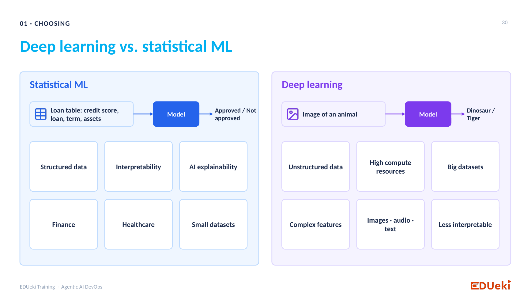
Deep learning vs. statistical ML
Statistical ML (linear regression, logistic regression, decision trees) works well for small, structured, simple data, such as the loan table or house prices. It struggles with big, complex or unstructured data, such as images, audio and text: for example, asking a model what an image shows. For those, you need deep learning, which uses neural networks.
2. The idea: add hidden layers
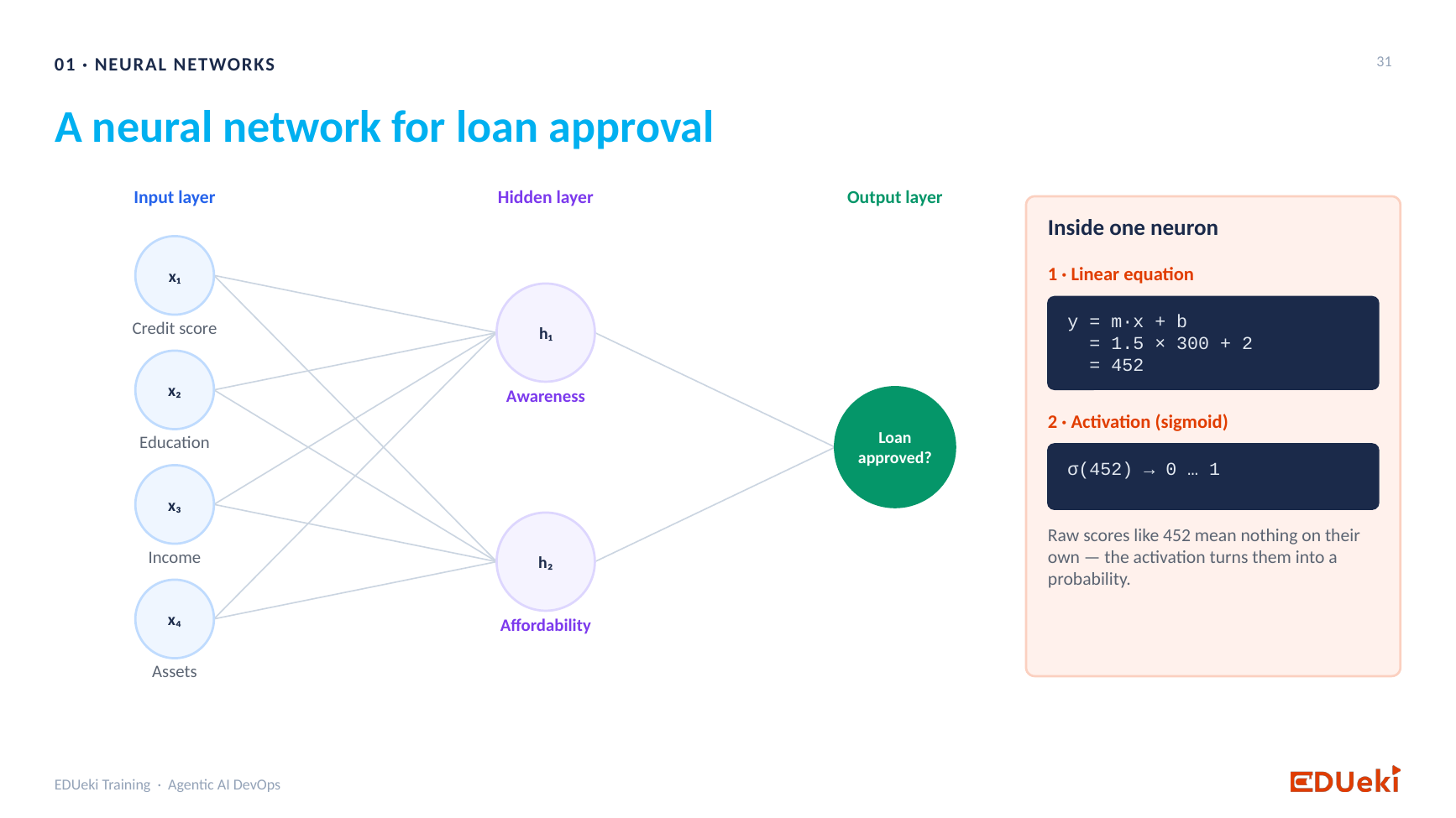
A neural network for loan approval
In statistical ML, the features x go straight to the prediction y, using m·x + b. That is a linear equation, and if the data is not close to linear, the accuracy is limited.
Neural networks add a middle step. Take the loan example with four inputs: credit score, education, income and assets.
- Instead of deciding the loan directly, first calculate two intermediate scores. For example, an awareness score (how well the applicant understands loans) based mostly on credit score and education, and an affordability score (can they repay?) based mostly on income and assets.
- Every input still feeds both scores, but with different weights.
- The final decision is made from these two scores, not from the raw inputs.
Analogy: instead of one loan manager reviewing the application, two junior managers each produce a score, and a senior manager decides from their scores. More scrutiny means fewer wrong decisions.
In a real network we do not know what each middle score “means”. Each neuron just produces a score that helps the next layer.
3. Neuron, perceptron and network
| Term | Meaning |
|---|---|
| Neuron | The smallest model: it takes inputs, applies learned weights and a bias in m·x + b, and (for classification) an activation function, and gives an output. It is what we called an “ML model” before |
| Perceptron | A neuron that has an activation function to produce its final score |
| Neural network | Several neurons working together |
| Layers | Input layer (the features), hidden layers (in the middle), output layer (the prediction) |
| Feed-forward network | Each layer passes its results forward to the next layer, one direction only |
- Every neuron in one layer sends its output to every neuron in the next layer, each with its own weight.
- Each neuron has its own equation and weights. In a neural network we do not call them “logistic regression” or “decision tree”. Those names belong to statistical models.
- The weights and bias are learned during training. At inference, the network simply applies them.
4. You design the network
With statistical ML you pick an algorithm from scikit-learn and give it data. With a neural network you design the architecture:
- how many hidden layers,
- how many neurons in each layer,
- which activation function each layer uses.
There is no fixed answer: try one hidden layer with four neurons, then two layers, and see which gives the best accuracy. It is experimentation again.
5. Activation functions
A linear equation gives any number, such as 452. For a classification, you need a probability, so you pass the number through an activation function. A regression output needs no activation function.
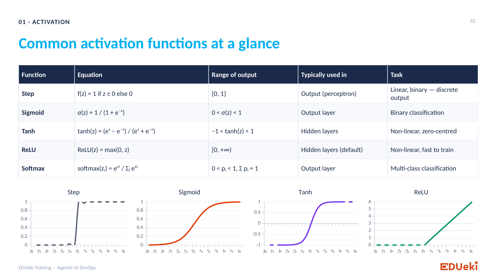
Common activation functions
They add up to 1, and the highest winsReLUHidden layers (the common default)Passes positive numbers through and turns negatives into 0.
Fast to trainStepRarely usedOutputs only 0 or 1TanhHidden layers, in some casesSqueezes a number into -1 to 1
| Function | Where You Use It | What It Does |
|---|---|---|
| Sigmoid | Output layer, binary classification | Converts a number into a value between 0 and 1, representing the probability of class 1. |
| Softmax | Output layer, multi-class classification | Converts scores into a probability distribution across all classes. |
Sigmoid example. If a transaction scores 0.8 on the sigmoid, there is an 80% chance it is fraud (class 1) and so a 20% chance it is not. With a decision boundary of 0.5 the answer is class 1. You can set a different boundary, such as 0.8, if you want to be stricter.
Softmax example. For an article that could be business, international, finance or banking, softmax might give 0.50, 0.20, 0.15 and 0.15. They add up to 1, and the highest (business) is the prediction.
import math

def sigmoid(z):
    return 1 / (1 + math.exp(-z))

x, w, b = [0.8, 0.9], [0.5, 0.3], 0.1       # inputs, weights, bias
z = sum(wi * xi for wi, xi in zip(w, x)) + b   # m1*x1 + m2*x2 + b = 0.77
print(round(sigmoid(z), 3))                    # 0.684  -> class 1 at the 0.5 boundary
A good default: ReLU in the hidden layers, sigmoid (binary) or softmax (multi-class) in the output layer. You only tell the network which function to use. It already knows the maths. In statistical ML the activation is built in and you never choose it.
6. How a neural network learns
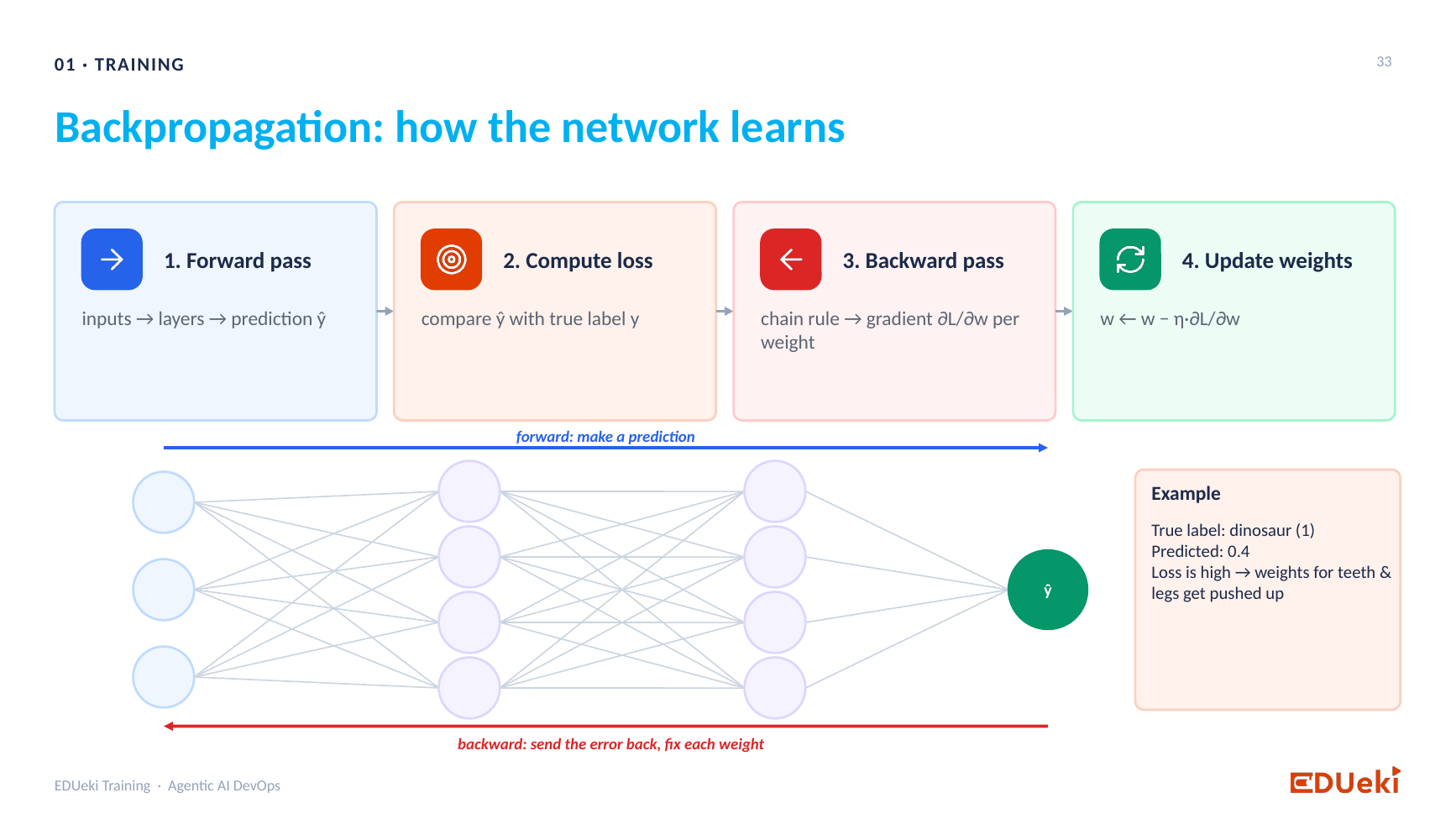
Backpropagation: forward pass, loss, backward pass, update weights
Training uses the same ideas as before, now applied to a network. Imagine a network that classifies an image:
- Start with random weights in every neuron. You do not supply them.
- Forward pass: the inputs go through the layers. Each neuron applies
m·x + band its activation function, and passes its score on. The output layer produces a prediction. - Compute the loss: compare the prediction with the truth from the dataset. If it is wrong, there is a loss.
- Backward pass: send the loss back through the previous layers, so each neuron knows how to adjust its weights.
- Update the weights and repeat. Each full round is an epoch. This is gradient descent, as in the earlier sessions. Training stops when the loss is minimal.
In statistical ML all of this was built in. In a neural network, you configure it.
7. What you configure
| Setting | Meaning |
|---|---|
| Layers and Neurons | Defines the structure and shape of the neural network. |
| Activation Function | Determines how each neuron transforms its input, as discussed above. |
| Loss Function | Measures how far the model’s predictions are from the actual values. For example, MSE is suitable for predicting numerical values such as house or stock prices, while Binary Cross-Entropy is suitable for binary classification, such as spam or not spam. |
| Learning Rate | Determines how large each adjustment to the weights is during training. Too small makes training slow, while too large can overshoot the optimal values. A good value is found through experimentation, such as 0.1 or 0.001. |
| Optimizer | Defines the algorithm used to update the network’s weights based on the gradients and learning rate. Examples include SGD, Adam, and RMSprop. |
Statistical ML models also use a loss function, a learning rate and an optimizer, but they are built in and you cannot control them. In deep learning you control them, which is why you can tune the network for your own data.
The next session builds a neural network in code.
Summary
Key takeaways
- Statistical ML suits small, structured data. Deep learning suits big, complex and unstructured data.
- A neuron is a small model (
m·x + bplus an activation). A neural network has an input layer, hidden layers and an output layer. - Hidden layers calculate intermediate scores that make the final prediction more accurate.
- Sigmoid is for binary output, softmax for multi-class output, and ReLU for hidden layers. Regression output needs no activation.
- Learning: forward pass, loss, backward pass, update weights, repeated for many epochs.
- You configure the layers, neurons, activation functions, loss function, learning rate and optimizer, and you find them by experiment.
Quick revision
| Term | Meaning |
|---|---|
| Neuron | A small computational unit consisting of weights, bias, and an activation function. |
| Hidden Layer | A layer positioned between the input layer and the output layer. |
| Feed-forward | Information flows from one layer to the next in a single direction, from input to output. |
| Activation Function | Transforms a neuron’s weighted input into an output value. |
| Loss Function | Measures the difference between the model’s predictions and the actual values. |
| Learning Rate | Determines the size of each weight adjustment during training. |
| Optimizer | The algorithm that updates the model’s weights to minimize the loss. |
| Backpropagation | Propagates the error backward through the network to calculate gradients and adjust the weights. |
Remember: a network is layers of simple neurons, and training is repeated correction of their weights.