
Agentic AI DevOps: ML Training – Classification Model (Loan Approval)
Recap of the previous session
- With many features, there is one weight per feature and a single bias.
- Plot features against the target to see which matter, and one-hot encode categorical data so the model only sees numbers.
- Never test on the training data. Split it with
train_test_split, randomly, with arandom_state. - The model is judged on the test set with a score such as R². A score of about 0.75 was not good enough, so you experiment.
In this session
- The classification use case: loan approval
- Analysing the dataset:
info,describeand unique counts - Cleaning and feature engineering: spaces, useless columns, duplicates, missing values, combining columns
- Encoding two-category columns, and scaling big numbers with
log - Splitting into
Xandy, training a logistic regression model, and measuring accuracy
In one sentence: most of the work in a real ML project is preparing the data. Once it is clean and numeric, training is the same few lines as before.
1. The use case: loan approval
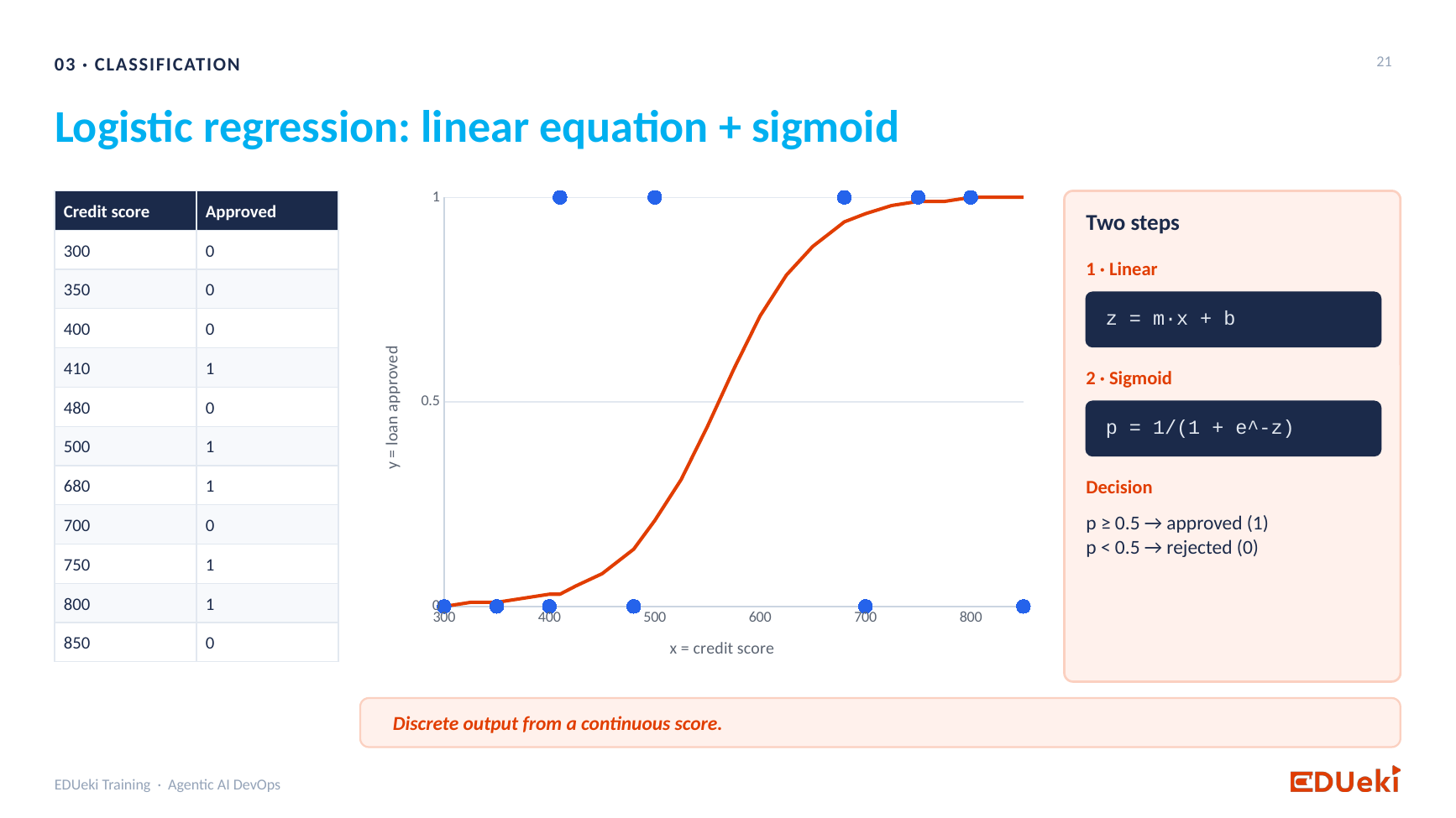
Logistic regression: a linear equation plus the sigmoid
Think of how a loan used to work: you fill in a form, a manager reviews it, and you wait a few days. Now an ML model reviews the application and answers immediately. For that, the model is trained on past applications.
The dataset has one row per previous applicant: number of dependents, education, self-employed (yes or no), annual income, loan amount, loan term, credit score, four asset values (residential, commercial, luxury, bank), and the loan status (approved or rejected).
- It is structured data, and supervised learning, because the loan status (the target) is in the data.
- Because the answer is a category, this is a classification problem.
2. Analyse the data first
import pandas as pd

data = pd.read_csv("../data/loan_data.csv")
data.shape        # (4270, 13)
data.info()       # types
data.head()
data.describe()   # statistics
- About 4,270 past applicants and 13 columns.
info()shows that education, self-employed and loan status are strings: categorical data that must be encoded.describe()gives the count, minimum, maximum, mean and quartiles for each numeric column. For the credit score, the minimum is 300, the maximum is 900 and the mean is about 600. This tells you whether the data is balanced. For example, you would not want nearly all credit scores to be 300.
You do not need to plot every feature again. You did that for regression, and the data scientists normally handle it.
3. Cleaning and feature engineering
The data you receive is never ready. These are the steps used here. Not every dataset needs all of them: analyse first, then decide.
a. Remove leading spaces from the column names
The column names start with a space, so data["loan_status"] fails with a key error.
data.columns = [i.strip() for i in data.columns]
b. Drop a feature that cannot help
data.nunique() shows the number of unique values per column. The loan ID has 4,269 unique values for about 4,270 records: every applicant has a different one, so there is no pattern to learn. Credit score has about 600 unique values and repeats across applicants, so it can carry a pattern. Remove features that do not influence the target. They only add complexity.
data.drop(columns=["loan_id"], inplace=True)
inplace=True updates the original DataFrame. Without it, the original is not changed.
c. Remove duplicate records
data.duplicated().sum()
data.drop_duplicates(keep="first", inplace=True)
Duplicates give some applicants extra weight and dominate the training, like practising the same question ten times.
d. Remove spaces from the categorical values
Text values often have leading spaces too (” Graduate”). Numbers do not.
data["education"] = data["education"].str.strip()
data["self_employed"] = data["self_employed"].str.strip()
data["loan_status"] = data["loan_status"].str.strip()
e. Handle missing values
data.isnull().sum() # credit_score has 4 missing values
Training needs a value everywhere. You can delete the affected rows, or fill them. You cannot get the real credit scores, so fill with the average (about 600):
data["credit_score"] = data["credit_score"].fillna(data["credit_score"].mean())
With 4 missing values out of about 4,000 the effect is small. If many were missing, it would matter. Train both ways and compare the accuracy: that is an experiment.
f. Combine columns
The four asset columns describe the same thing. The bank only needs the total, so combine them and drop the four originals. Fewer features means simpler training.
data["total_assets"] = (data["residential_assets_value"] + data["commercial_assets_value"]
                        + data["luxury_assets_value"] + data["bank_asset_value"])
data.drop(columns=["residential_assets_value", "commercial_assets_value",
                   "luxury_assets_value", "bank_asset_value"], inplace=True)
The dataset is now down to 9 columns.
g. Encode the categorical columns
In session 6, one-hot encoding suited job title because it had five categories. Here each column has only two categories, so a simple 0/1 mapping is enough (this is called label encoding).
data["education"] = data["education"].map({"Graduate": 1, "Not Graduate": 0})
data["self_employed"] = data["self_employed"].map({"No": 1, "Yes": 0})
data["loan_status"] = data["loan_status"].map({"Approved": 1, "Rejected": 0})
The meaning is not lost, only the representation changes. Scikit-learn also has a LabelEncoder, but it chooses which category becomes 0 or 1 for you. Writing the mapping yourself lets you decide that Approved = 1.
Remember these mappings. When the model is used later, the same encoding must be applied to new data.
h. Scale down large numbers
Annual income, loan amount and total assets are in the millions, while other features are tiny. The model struggles to find a pattern with such different sizes. The model does not care what the number means. It only looks for patterns, so you can represent the numbers on a smaller scale without losing the pattern. Use NumPy’s log:
import numpy as np

data["income_annum"] = np.log(data["income_annum"])
data["loan_amount"] = np.log(data["loan_amount"])
data["total_assets"] = np.log(data["total_assets"])
Analogy:
1/2 + 1/2and0.5 + 0.5are the same sum, but the second is easier to compute. It is the same value in an easier form.
4. Features and target
X = data.drop(columns=["loan_status"])   # everything except the answer
y = data["loan_status"]                  # approved (1) or rejected (0)
x and y are only variable names. They are the standard notation, so anyone reading your code understands them. At inference time you send only the input features (like X) and the model returns the loan status.
5. Training and measuring accuracy
from sklearn.model_selection import train_test_split

x_train, x_test, y_train, y_test = train_test_split(X, y, test_size=0.2, random_state=42)
An 80/20 split: 80% of the records to train and 20% to test.
For classification, scikit-learn offers several algorithms. Here we use logistic regression. (Session 5 used linear regression, because that was a regression problem.) The steps are the same: import, create the object, fit, predict.
from sklearn.linear_model import LogisticRegression

model = LogisticRegression()
model.fit(x_train, y_train)                # training
predictions = model.predict(x_test)        # 1 = approved, 0 = rejected
To judge the model, compare the predictions with the truth (y_test) using accuracy_score:
from sklearn.metrics import accuracy_score

accuracy_score(y_test, predictions)        # about 0.91
An accuracy of about 91% means that out of 100 applicants, about 91 get the correct decision and about 9 do not. If this is not good enough, go back to the data, features or algorithm. How to improve it is the next session.
6. A learner’s question: how does it work for a new applicant?
A new applicant has no loan status yet. Think of a loan manager: they study past applications to learn when loans were approved or rejected. When a new applicant arrives, they decide using what they learned. The model does the same. It trains on previous applicants (with the answers) and then predicts the loan status for a new applicant from the input features alone.
Summary
Key takeaways
- Loan approval is a binary classification problem, using supervised data.
- Analyse the data first:
shape,info,describe,nunique. - Clean it: strip spaces, drop useless columns, remove duplicates, fill missing values, combine similar columns.
- Encode categories as numbers: a 0/1 mapping for two categories, one-hot for more.
- Scale down big numbers with
log. - Split into
Xandy, thentrain_test_split,LogisticRegression,fit,predictandaccuracy_score. - About 91% accuracy on the first attempt.
Quick revision
| Term | Meaning |
|---|---|
| Binary classification | Two possible answers (approved or rejected) |
nunique() |
Number of unique values in each column |
| Duplicate | The same record repeated, which gives it extra weight |
| Missing value | An empty cell. Delete the row or fill it (for example with the mean) |
| Label encoding | Mapping two categories to 0 and 1 |
np.log |
Compresses large numbers into a smaller range |
| Accuracy | Share of predictions that match the truth |
Remember: clean the data, make it numeric, then train.